
Material testing provides the experimental foundation required to understand and model the dynamic response of tire compounds. Rubber and other polymer-based materials cannot be represented reliably through a single elastic constant because their stiffness and energy dissipation change with excitation frequency, temperature and loading conditions.
The scientific study examined in this article investigates how experimental measurements can be transformed into a robust mathematical representation of viscoelastic materials. Its central contribution is a nonlinear generalized fractional Maxwell model designed to reproduce storage modulus and loss factor across broad frequency-temperature ranges and for materials with substantially different dynamic responses.
The study was validated on ten different materials intended for tire-related applications. It also investigated whether a complete material response could be reconstructed from selected experimental regions instead of requiring measurements across the entire available frequency range.
This article therefore focuses specifically on material characterization, material analysis and experimental-data efficiency. For a broader explanation of the nonlinear formulation, pole-zero representation and complete mathematical framework, see the VESevo article on nonlinear modeling of viscoelastic materials for tire applications.
The material-oriented approach is relevant to tire manufacturers, testing laboratories, compound engineers and simulation specialists who need to convert measured material properties into models suitable for finite-element analysis, structural dynamics, tire simulation and product-lifecycle assessment.
Rubber Material Testing: DMA and Dynamic Response
Rubber materials can be investigated through static, quasi-static, transient and dynamic testing procedures. Each method provides information about a different part of the material response.
Static and quasi-static tests apply slowly varying forces or deformations. Transient procedures include impact, creep and stress-relaxation experiments. Dynamic tests instead expose a material sample to oscillating stress or strain and measure the amplitude and phase of the resulting response.
Dynamic Mechanical Analysis, or DMA, is one of the most established methods for testing polymeric materials. It measures the quantities needed to describe how a material stores and dissipates energy under periodic loading.
For the experimental campaign considered in the paper, the ten materials were tested through DMA using:
- a tensile test configuration with horizontal orientation;
- a reference frequency of 1 Hz;
- a temperature sweep from −50 °C to 120 °C;
- a temperature ramp of 1 °C per minute;
- The paper reports a strain setting of 0.1% and an oscillatory strain-control amplitude of 0.05%.
- a static force of 2 N.
All samples were tested under equivalent conditions, allowing differences among the compounds to be attributed to their own materials’ characteristics rather than to changes in the experimental procedure.
Conventional DMA generally requires prepared specimens and is usually destructive. The study also notes the emergence of non-destructive methods capable of evaluating finished products. VESevo, for example, identifies viscoelastic characteristics by studying the dynamics of a freely bouncing rod without cutting a sample from the tire.
This relationship between testing and modeling is explored further in the VESevo article on non-destructive testing and viscoelastic characterization.
Material Characterization Through Storage Modulus and Loss Factor
Material characterization requires quantities that distinguish the elastic and dissipative components of the response. When sinusoidal stress is applied to a viscoelastic solid, the resulting strain occurs at the same frequency but with a phase delay caused by internal energy dissipation.
The dynamic response is represented through the complex modulus:
E* = E′ + jE″
The storage modulus E′ describes the elastic contribution, while the loss modulus E″ represents the dissipative contribution. Their ratio defines the loss factor:
tan δ = E″ / E′
The material’s storage modulus indicates how much elastic energy can be retained during each deformation cycle. The loss factor describes the relative importance of damping and hysteretic dissipation.
These measurements are essential because the material viscoelastic properties are not constant. E′, E″ and tan δ depend on the frequency of excitation and on the instantaneous temperature of the sample.
A useful model for material simulation must reproduce both storage modulus and loss factor simultaneously. Fitting only one of these quantities may produce an incomplete or physically misleading representation of the compound.
Material Behaviour Across Frequency and Temperature
The material behaviour of polymers is closely related to the mobility of their molecular chains. At low excitation frequencies, the chains have sufficient time to reorganize under the applied load. The response is therefore associated with the rubbery region.
At high frequencies, molecular reorganization becomes progressively restricted. The material moves toward a glass-like response, and its effective stiffness increases.
Temperature produces a related effect. Increasing temperature enlarges the available intermolecular free volume, facilitating molecular movement and generally reducing storage modulus at a fixed frequency.
The time-temperature superposition principle connects these two effects. Measurements acquired over a limited frequency interval at several temperatures can be shifted to reconstruct a master curve covering a much wider operating domain.
This is particularly important for tire applications because commercial test equipment may not directly reach every frequency generated during road excitation. A model must therefore represent the material’s behaviour outside the directly measured range while remaining consistent with the available experimental evidence.
From Ideal Materials to Real Polymeric Materials
Classical rheological descriptions often begin with ideal materials. A perfect spring represents instantaneous elastic behaviour, while a perfect dashpot represents purely viscous deformation.
Real polymeric materials are more complex. Their response reflects molecular-chain length, intermolecular forces, curing, crystallinity, polymers, oils, resins, additives and manufacturing treatments.
In an idealized viscoelastic response, the storage modulus changes smoothly between low- and high-frequency plateaus, while the loss factor follows a bell-shaped curve around the transition region. Real compounds may instead exhibit additional slope changes and inflection points.
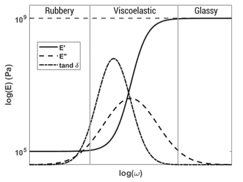
The distinction between ideal and real behaviour explains why simple linear models can be effective only over restricted intervals. The broader behaviour of materials used in tire applications may require a formulation capable of adapting to multiple transition patterns.
This does not mean that every material requires a nonlinear model. Materials with regular transition zones may already be described accurately by a conventional fractional formulation. Nonlinear flexibility becomes valuable when experimental curves show complex or non-uniform variations.
Material Analysis: Comparing Linear and Nonlinear Viscoelastic Models
Material Analysis in the study compares the conventional Generalized Fractional Maxwell Model, or GFMW, with the proposed Nonlinear Generalized Fractional Maxwell Model, or NLGFMW.
The classical model combines fractional Maxwell cells with an isolated spring. It provides an efficient representation of many viscoelastic materials, but it can struggle when the storage modulus contains marked changes in slope.
Another difficulty concerns multi-objective calibration. The model must approximate storage modulus and loss factor at the same time. Giving priority to one curve can improve its fit while worsening the prediction of the other.
The proposed nonlinear model introduces frequency dependence into the isolated stiffness term K0. This additional flexibility modifies the magnitude and trend of the storage modulus without introducing an inconsistent change in the predicted phase response.
The comparison reported in the paper shows that the nonlinear formulation is especially advantageous for materials whose experimental curves differ substantially from smooth idealized trends.
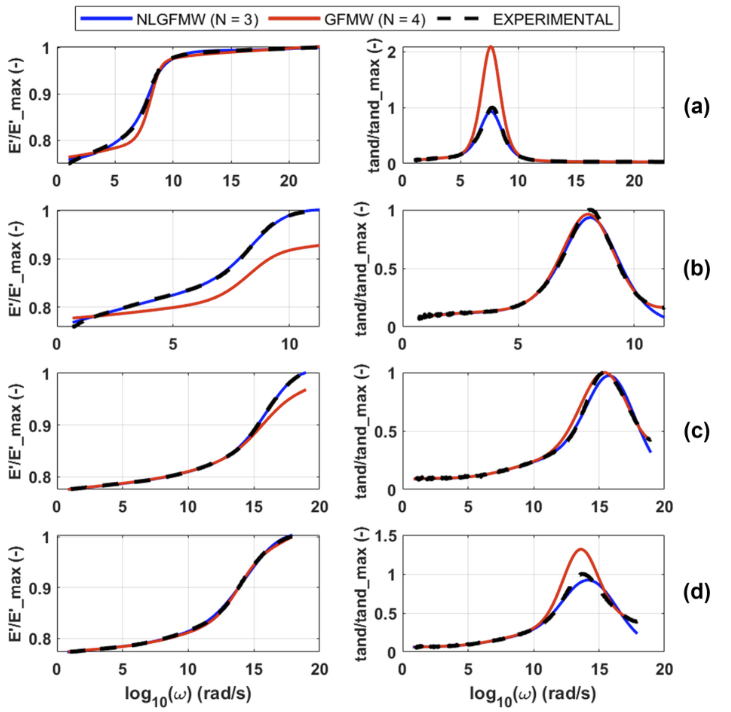
The improvement is particularly evident for materials with less regular viscoelastic trends. Comparing the three-element NLGFMW with the four-element GFMW, the storage-modulus MAPE decreases from 31.491% to 5.204% for Compound E, from 24.652% to 1.907% for Compound F and from 19.322% to 3.118% for Slab D.
For Compounds A, B and C, which have regular and clearly marked transition zones, the traditional fractional model already provides excellent results. For the other seven materials, the nonlinear approach improves the simultaneous prediction of storage modulus and loss factor.
This result supports an adaptive strategy: use the simplest model that satisfies the required accuracy, activating nonlinear behaviour only when the experimental material properties make it necessary.
Material Modeling with Fractional Maxwell Elements
Material modeling translates experimental curves into a constitutive law that can be implemented in engineering calculations. Classical Maxwell and Kelvin–Voigt models combine springs and dashpots, but their simple forms cannot reproduce broad frequency-dependent behaviour.
Generalized models connect several elements to represent multiple characteristic times. Their main disadvantage is the large number of differential equations and parameters required for calibration.
Fractional models replace the conventional dashpot with a spring-pot. Its derivative order lies between zero and one, allowing the element to reproduce intermediate elastic-dissipative behaviour.
For the solid material considered in the paper, fractional Maxwell cells are arranged in parallel with an isolated stiffness. This produces a compact constitutive representation capable of describing reversible creep, elastic storage and hysteretic dissipation.
These viscoelastic materials models are particularly useful when material laws must be implemented in finite-element analyses or simulation environments where numerical efficiency and parameter identifiability are important.
Frequency-Dependent Stiffness in the NLGFMW Model
The key extension introduced by the authors is a stiffness function K0(ω) that varies with excitation frequency. The function is constructed from two Gaussian components centered near the glass-transition frequency.
Five parameters govern its scale, width, peak, asymmetry and behaviour away from the transition zone. The additional term increases flexibility without requiring a separate nonlinear function for every Maxwell cell.
The resulting material viscoelastic behaviour remains mathematically compatible with the pole-zero formulation used for parameter identification.
Pole-Zero Identification and Multi-Objective Model Calibration
Direct calibration of spring stiffnesses and spring-pot coefficients can be difficult because the parameters may differ substantially in magnitude. Optimization can converge toward a local solution that depends on the initial parameter values.
The pole-zero representation reduces this difficulty by imposing a physically consistent alternation between pole and zero frequencies. Once these frequencies are identified, the corresponding Maxwell parameters can be reconstructed.
The calibration is treated as a multi-objective problem because storage modulus and loss factor must both be reproduced. The NSGA-II algorithm is used to search for suitable trade-off solutions, while the Mean Absolute Percentage Error quantifies agreement with the experimental curves.
The general workflow begins with four fractional Maxwell cells and a constant K0. When the errors for both dynamic quantities remain below a 10% threshold, the simpler formulation is accepted. Otherwise, the frequency-dependent parameters are activated.
A subsequent reduction to three cells is attempted to determine whether an equally acceptable model for material representation can be obtained with fewer parameters and shorter computation time.
Material Characteristics Across Ten Experimental Samples
The ten materials were selected to represent a broad range of dynamic responses without disclosing their confidential chemical composition. They consist of six compounds and four slab materials.
The samples differ in:
- glass-transition frequency;
- maximum loss-factor value;
- stabilized storage modulus in the glassy region;
- strength and regularity of their transition zones;
- low- and high-frequency slope behaviour.
Compounds A, B and C show marked and regular transition regions together with comparatively high glassy plateaus. Compounds D, E and F show less pronounced low-frequency transitions and different combinations of loss factor and storage modulus.
Slabs A, B, C and D are characterized by higher glass-transition frequencies and lower relative storage-modulus and loss-factor values. These differences make the dataset suitable for testing whether the model can adapt to substantially different material behaviour.
Material Model Accuracy and Computational Efficiency
The NLGFMW formulation was evaluated with three, four and five fractional elements. These configurations contain 14, 17 and 20 parameters respectively when the nonlinear stiffness function is active.
Across the complete experimental dataset, all three versions provided satisfactory results, with maximum errors of approximately 7% for storage modulus and loss factor.
Increasing the number of cells generally improves fitting accuracy, but it also increases computational load and can complicate parameter identification. In some cases, the five-element configuration performed slightly worse than the four-element model because the available data were insufficient to identify the larger parameter set efficiently.
The study therefore identifies the four-element NLGFMW as the most balanced general configuration. It offers a useful compromise among accuracy, adaptability and computational complexity.
The three-element version remains attractive when faster evaluation is required. Its average calibration time was approximately 1.9 seconds, compared with 2.6 seconds for the four-element model and 3.3 seconds for the five-element configuration on the computing platform used by the authors.
The three-element model was, on average, approximately 48% faster than the five-element version while still producing comparable errors. The authors identify this as a potential advantage for real-time evaluation or material-monitoring applications.
Material Testing with Limited Experimental Data
Extending experimental acquisition across a very broad frequency range increases test duration, equipment requirements and cost. One of the most practically relevant parts of the study therefore concerns calibration from a reduced number of data zones.
The selected regions include:
- the low-frequency storage-modulus plateau;
- the region around the glass transition and loss-factor peak;
- the high-frequency storage-modulus plateau, when available.
These zones contain information about the material far from the glass transition and within the transition region. They are therefore particularly informative for identifying the nonlinear stiffness parameters.
For Compounds A, B, C and D, data were available for all three regions. For the other materials, the available measurements ended shortly after the loss-factor peak, so calibration used only the low-frequency plateau and transition region.
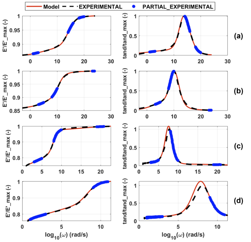
Using three selected zones covering approximately 20–30% of the complete experimental dataset, the model reproduced the broader response with promising accuracy.
The resulting MAPE values remained below 10% in almost every case. The exception was the loss-factor prediction for Slab D, which reached approximately 15% and was calibrated using only two experimental regions.
This result does not imply that extensive testing is unnecessary in every application. It demonstrates that carefully selected measurements can provide more information than a larger but poorly distributed dataset.
For tire makers that can estimate glass-transition temperature from the compound formulation, the approach may support more targeted testing strategies and reduce resource consumption during preliminary material characterization.
Engineering Value of Viscoelastic Material Modeling for Tire Applications
A reliable representation of material properties supports several engineering workflows. Purely elastic models may be insufficient when the product response depends on damping, frequency, temperature or aging.
Potential applications include:
- finite-element analysis of tire and polymer components;
- complex eigenvalue and vibration analyses;
- comparison of rubber compounds;
- temperature- and frequency-dependent tire models;
- product-design and material-selection studies;
- performance forecasting over a product lifecycle;
- monitoring changes caused by aging or operating conditions;
- reduced experimental campaigns based on selected data zones.
The study does not claim that mathematical modeling eliminates the need for physical tests. Experimental data remain the basis of the identification procedure. The model increases their engineering value by transforming measured curves into a continuous and computationally usable representation.
This relationship is relevant to other VESevo investigations concerning non-destructive tire measurement and material performance characterization and rubber viscoelasticity, abrasion and road contact.
Limits of the Material Modeling Approach
The results are promising, but several boundaries should be considered:
- The ten-material dataset is broad in mechanical response but does not disclose detailed chemical composition.
- The experimental data are normalized for confidentiality.
- The study focuses on small-amplitude DMA characterization rather than large-strain tire deformation.
- The nonlinear term depends on frequency and is not presented as a complete model of every possible material nonlinearity.
- The reduced-data method requires representative measurements around the most informative regions.
- Limited calibration data produced a loss-factor error above 10% for one material.
- Product-level performance predictions still require structural modeling and application-specific validation.
The model should therefore be interpreted as a versatile constitutive representation of frequency-temperature dependent material viscoelastic behaviour, not as a replacement for all compound-specific and product-level testing.
Frequently Asked Questions About Material Testing and Analysis
What is material testing for viscoelastic tire compounds?
Material testing measures how a tire compound responds to controlled stress, strain, frequency and temperature. The resulting data describe stiffness, damping and transition behaviour.
What does DMA measure?
Dynamic Mechanical Analysis measures quantities such as storage modulus, loss modulus and loss factor while the sample is subjected to oscillatory deformation.
Why does viscoelastic behaviour depend on frequency?
At lower frequencies, polymer chains have more time to reorganize. At higher frequencies, molecular movement is restricted, producing a stiffer and more glass-like response.
Why does temperature affect the viscoelastic behaviour of rubber materials?
Temperature changes molecular mobility and free volume. This shifts the frequency-dependent viscoelastic response and modifies storage modulus and damping.
What is the difference between GFMW and NLGFMW?
The NLGFMW model extends the conventional fractional Maxwell formulation with a frequency-dependent stiffness term, improving its ability to reproduce complex storage-modulus trends.
Is the nonlinear model always necessary?
No. The conventional fractional model performed well for materials with regular and clearly defined transition zones. Nonlinear flexibility was most useful for less regular responses.
How many fractional elements provide the best balance?
The study evaluates three-, four- and five-element configurations. Four elements provide the preferred general balance between accuracy and complexity, while three can provide faster results with comparable errors.
Can the model work with limited experimental data?
Yes. Selected measurements from the low-frequency plateau, glass-transition region and high-frequency plateau reproduced the broader material response with errors below 10% in almost every analyzed case.
Does limited-data calibration replace complete material testing?
No. It provides a resource-efficient alternative when the selected data cover physically informative regions and the resulting model is validated against the intended application.
Can VESevo support non-destructive material characterization?
VESevo provides non-destructive dynamic characterization of finished products such as tires and can supply viscoelastic information without extracting a conventional DMA specimen.
Who can use these viscoelastic materials models?
They are relevant to material engineers, testing laboratories, tire manufacturers, simulation specialists and researchers working with polymeric components.
Scientific Source
This article is based on: Sakhnevych, A.; Maglione, R.; Suero, R.; Mallozzi, L. Nonlinear mathematical modeling of frequency-temperature dependent viscoelastic materials for tire applications. Nonlinear Dynamics, 2024. DOI: 10.1007/s11071-024-10175-z.
The original publication is distributed under the Creative Commons Attribution 4.0 International licence.
Editorial note: This article provides a material-testing and analysis-focused interpretation of the cited scientific study. It does not replace compound-specific laboratory testing, constitutive-model validation, structural simulation or product-level engineering assessment.