
Rubber wear is governed by the interaction among material viscoelasticity, road texture, temperature, sliding conditions and repeated mechanical loading. For tire compounds, material removal cannot be represented reliably as a constant function of mileage because the mechanical state of the tread changes continuously during operation.
The scientific model examined in this article describes wear at the material level. It follows the evolution of the rubber matrix, the stresses generated beneath the contact surface and the accumulation of fatigue damage inside discrete tread volumes. Temperature and excitation frequency are used to update the instantaneous properties of the compound before the local wear calculation is performed.
This material-focused analysis complements the VESevo article describing the complete tire wear model based on viscoelasticity, road roughness and thermodynamic state. That article explains the multidisciplinary model architecture and its vehicle-level validation. The present analysis concentrates instead on rubber viscoelasticity, abrasion, rough-surface contact and fatigue-driven material removal.
The distinction is important because different rubbers can respond very differently to the same nominal load. Their stiffness, energy dissipation, fatigue resistance and surface response depend on temperature, excitation frequency and operating history.
Rubber Wear and Abrasion at the Material Scale
Tire tread wear has consequences for performance, safety, operating cost and non-exhaust particle emissions. In motorsport, tread degradation can reduce the ability to maintain grip throughout a stint. In passenger and heavy-duty applications, wear affects service life, safety margins and the amount of material released into the environment.
Several mechanisms can contribute to polymer wear, including adhesion, abrasion, fatigue and surface detachment. For tire tread compounds, rubber abrasion is often the dominant description because repeated contact with pavement asperities progressively removes material from the tread.
The paper treats fatigue-generated material removal as wear abrasion, or simply wear. Local contacts are repeated many times while the tire rolls and slides, producing cyclic stresses and strains. Cracks can initiate and propagate until small volumes detach from the tread.
This process is not governed exclusively by frictional power. The effective wear rate also depends on the instantaneous rubber characteristics, the thermal state, the road excitation frequency and the stress history inside the compound.
Rubber Characterization: Viscoelastic Master Curves and Compound Response
Accurate Rubber Characterization is the foundation of the proposed wear calculation. A tire tread cannot be represented by one fixed elastic modulus because a rubber material combines elastic and viscous behaviour.
The dynamic response is represented by the complex modulus:
E* = E′ + iE″
The storage modulus E′ describes the elastic component of the response, while the loss modulus E″ describes the dissipative component. Their ratio defines the loss factor:
tan δ = E″ / E′
Storage modulus and loss factor vary with both excitation frequency and temperature. The same compound can therefore appear relatively compliant under one operating condition and considerably stiffer under another.
The five rubber compounds included in the validation dataset were evaluated through non-destructive VESevo technology. The resulting master curves describe differences in stiffness, transition behaviour and hysteretic dissipation among the compounds.
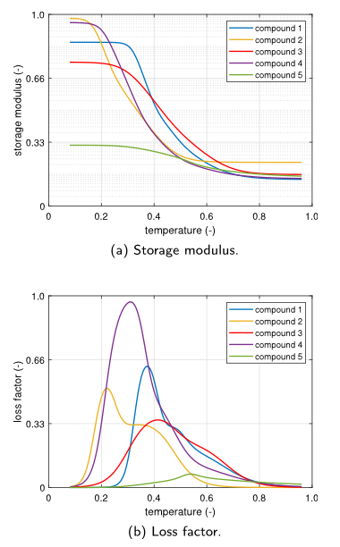
The use of measured material curves reduces the limitations associated with nominal compound data. This is particularly relevant during preliminary model development, when destructive laboratory characterization may require unavailable samples or specially manufactured specimens.
The role of non-destructive measurement is examined further in the VESevo analysis of tire testing and viscoelastic characterization.
Time-Temperature Superposition for Rubber Viscoelasticity
The time-temperature superposition principle extends the material response beyond the frequency and temperature limits directly covered by individual measurements. Experimental isotherms are shifted toward a selected reference temperature to construct broader master curves.
The horizontal shift is described through a temperature-dependent coefficient that follows the Williams-Landel-Ferry relationship. In the wear model, this allows E′, E″ and tan δ to be recalculated as the local temperature and excitation frequency change.
The model therefore does not assign one static set of properties to the tread. The instantaneous material state is reconstructed for each calculation node and operating condition.
Fractional Modeling of the Rubber Matrix
The frequency-dependent response of the rubber matrix is represented through a fractional Maxwell formulation. Fractional viscoelastic models can reproduce broad material transitions with a limited number of constitutive parameters.
This approach is computationally useful when the tread is divided into many nodes. Instead of storing a large pre-discretized database of every possible temperature-frequency combination, the required properties can be calculated analytically during the simulation.
A more detailed discussion of this approach is available in the VESevo article on nonlinear and fractional viscoelastic modeling for tire materials.
Rubber Analysis: Rough-Surface Contact and Internal Stress Fields
Rubber Analysis requires a connection between the measured compound properties and the mechanical conditions generated by the road. In the proposed formulation, pavement texture is converted into a set of rigid indenters acting on a viscoelastic semi-space.
Rubber – Rough Surface Interaction
The Rubber – rough surface problem is represented using road correlation lengths obtained from surface-profile and Power Spectral Density analysis. These quantities define the characteristic dimensions and spacing of the road-representative indenters.
The tire side of the contact is modeled as a Rubber – representative elastic semi-space. This idealization makes it possible to calculate indentation and subsurface stress while preserving the influence of the instantaneous viscoelastic modulus.
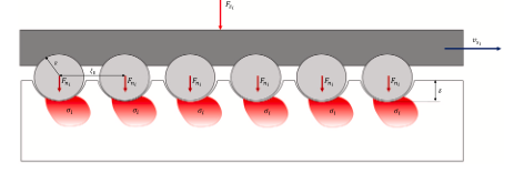
The characteristic excitation frequency is obtained from the local sliding velocity and the longitudinal road correlation length:
f = vs / ξ∥
This relationship connects vehicle kinematics with material behaviour. A change in sliding velocity or pavement wavelength changes the frequency at which the tread is excited and therefore modifies its effective stiffness and dissipation.
Stress Distribution in the Rubber – Road Contact Region
Within the Rubber – road contact region, the local pressure, friction coefficient and asperity dimensions determine indentation and stress distribution. Normal and shear stresses are evaluated beneath each representative indenter.
The response is not limited to the external rubber surface. Stress components extend through the tread thickness and influence the damage accumulated inside the complete rubber block.
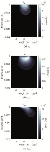
These internal stress fields provide the mechanical input for the fatigue-damage calculation. They create a direct link among road texture, contact pressure, local friction and the progressive removal of tread material.
The broader relationship between contact mechanics and friction is discussed in the VESevo study on tire friction and local contact-area modeling.
Rubber – Surface Interfacial Behaviour and Abrasion
Rubber – surface interfacial behaviour includes adhesion, local sliding, cyclic deformation and stress transmission between the compound and the pavement. These mechanisms are deeply interconnected during real tire operation.
The model does not attempt to separate adhesive and hysteretic friction into independent wear contributions. Instead, the forces responsible for friction generation are considered together as model inputs, while the viscoelastic state of the material is updated from temperature and frequency.
This choice distinguishes the formulation from a conventional rubber friction analysis designed primarily to decompose the total friction coefficient. Here, frictional forces are used to determine the local stress state that drives fatigue and material removal.
The approach is consistent with the difficulty of isolating individual friction and wear mechanisms under realistic operating conditions. Adhesion can contribute to surface detachment, while hysteretic deformation influences energy dissipation and subsurface stress. Both can affect the final abrasion state.
For a dedicated discussion of adhesive and viscoelastic friction mechanisms, see the VESevo analysis of tire adhesion, contact and viscoelasticity.
Rubber Performance: Temperature, Frequency and Damage Sensitivity
Rubber Performance in the wear calculation depends on the thermodynamic and mechanical history of the compound. The number of cycles required to reach local failure changes as temperature and excitation frequency change.
The tire thermal model calculates a three-dimensional temperature gradient through the tread and surrounding layers. Heat generation includes two principal contributions:
- hysteretic energy dissipation during repeated loading and unloading;
- heat produced by local sliding friction.
Road temperature, air temperature, tire structure, brakes, airflow and vehicle configuration contribute to the thermal boundary conditions. The resulting gradient is more informative than one surface-temperature value because the compound properties vary through the tread thickness.
Frequency is equally important. Road texture and sliding velocity define how rapidly the material is excited. Temperature and frequency together shift the storage modulus, loss factor and stress-life relationship used by the damage model.
Consequently, the same nominal stress does not always produce the same fatigue life. A compound can experience substantially different damage rates during warm-up, thermal steady state, free rolling or high-slip operation.
Rubber Control Volume and Cumulative Fatigue Damage
The tread is discretized into elementary material volumes. For every rubber control volume, the damage state is represented by a variable D ranging from zero to one.
The model starts from Miner’s linear cumulative-damage rule. The damage generated during each cycle depends on the number of cycles to failure under the current stress, temperature and frequency conditions.
The number of cycles to failure is therefore written as a function of temperature and excitation frequency rather than treated as a fixed material constant. This extension enables the fatigue model to follow the changing viscoelastic state of the compound.
The cumulative damage can be represented conceptually as:
D = ∫ dN / Nf(T,f)
When D reaches one, the elementary volume is considered detached. The node beneath it becomes the new contact node for the following calculation step. In this way, the model progressively reproduces tread-thickness reduction rather than applying one predetermined wear rate.
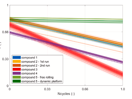
The stress-life curves form bundles rather than single fixed lines because the damage threshold changes with the thermodynamic state. Their slope is linked to intrinsic material properties, including hardness and elongation behaviour under glassy conditions.
Rubber Testing: Five Compounds Across Diverse Operating Conditions
Rubber Testing was performed using outdoor datasets from five tire specifications. The purpose was not merely to calibrate one compound but to evaluate the formulation across significantly different material and operating windows.
| Application | Material operating range | Tread temperature | Excitation frequency |
|---|---|---|---|
| Moderate-performance single-seater | Lower aerodynamic load and moderate sliding | 28–105 °C | 100–850 Hz |
| High-performance GT car | Higher loads and broad thermal range | 33–125 °C | 150–1000 Hz |
| Ultra-high-performance single-seater | High aerodynamic load and high slip | 60–130 °C | 250–1500 Hz |
| Production sports car | Passenger compound under moderate loads | 40–90 °C | 50–800 Hz |
| Heavy-duty truck | Very high normal load and lower slip frequency | 30–95 °C | 50–550 Hz |
The selected conditions expose the model to wide variations in compound stiffness, loss factor, contact stress and thermal state. The heavy-duty compound, for example, experiences the highest normal loads but lower excitation frequencies than the motorsport specifications.
This diversity is essential because a formulation validated only on one compound or one operating temperature cannot demonstrate general applicability to different rubber compounds and tire categories.
Rubber Measurement: Tread Thickness, Wear Channels and Rubber Mass
Rubber Measurement was based on tread-thickness inspection before and after the experimental sessions. At least two measurement states were available for each dataset, with one to three gauging positions per tire depending on its tread layout.
The measured positions were associated with the lateral ribs represented in the wear model. This allowed the remaining tread profile to be compared directly with the simulated wear channels.
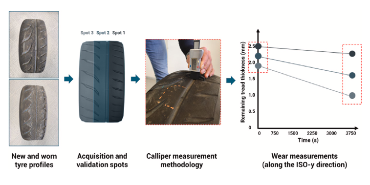
The model output can be expressed as remaining tread thickness, removed material volume or removed rubber mass. These outputs can support durability analysis, environmental assessment and the progressive updating of tire-dynamics models.
The use of physical tread measurements also prevents the model from being validated only through indirect quantities such as temperature or frictional power. Material loss is compared with an observable final wear state.
Additional context on tire and material measurements is available in the VESevo article on non-destructive tire measurement and performance characterization.
Experimental Validation of Rubber Wear Prediction
The simulated tread profiles were compared with the experimental remaining-thickness measurements for the five vehicle applications. The results show that the removal rate is generally nonlinear with running distance.
The average normalized final-wear errors were:
- 2% for the moderate-performance motorsport compound;
- 3% for the high-performance GT compound;
- 4% for the ultra-high-performance motorsport compound;
- 4% for the passenger-car compound;
- 4% for the heavy-duty compound.
The individual vehicle-corner errors ranged from 1% to 7%. Average errors remained below 5% for every application included in the dataset.
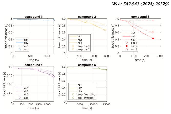
For two compounds, the experimental information also supported validation of the wear evolution with mileage rather than only the final state. For the remaining specifications, the validation primarily concerns the final measured tread condition.
The results demonstrate that the formulation can reproduce material removal across different compounds, road surfaces and thermodynamic conditions. They do not demonstrate that every microscopic abrasion mechanism has been identified independently.
Engineering Applications of Rubber Wear Modeling
The material-level formulation can be integrated into simulation environments with different degrees of spatial resolution. Detailed finite-element co-simulations can use local temperature, pressure and velocity distributions, while reduced real-time models can use average contact quantities.
Potential applications include:
- comparison of tread compounds under different thermal conditions;
- analysis of rubber abrasion on different road textures;
- prediction of remaining tread thickness;
- estimation of removed rubber volume and rubber mass;
- motorsport tire-management simulations;
- passenger and heavy-duty durability studies;
- real-time driver-in-the-loop simulation;
- onboard tire-state monitoring and control systems;
- updating of stiffness, friction and thermal models as wear progresses.
For high-performance applications, the model can complement statistical approaches based on telemetry and experimental wear data. An example is discussed in the VESevo article on tire wear prediction for high-performance vehicles.
Limits of the Rubber Wear Formulation
The current model has several limitations that define the boundaries of its application.
- Thermomechanical and chemical degradation effects on viscoelastic and thermal-diffusivity properties are not included.
- The contact-patch size, shape and complete kinematic response are not continuously updated as tread geometry changes.
- The preliminary thermal calibration assumes a constant wear level throughout the simulated temperature history.
- Detailed tire, compound and operating data remain confidential.
- Local pressure, temperature and velocity fields may require numerical estimation because they are difficult to measure directly during real-road operation.
- The validation does not isolate adhesive, hysteretic and fatigue wear contributions experimentally.
These limitations mean that the model should be calibrated and validated within the intended operating range. They do not remove its main advantage: the ability to connect measured material properties, rough-surface contact, temperature and cumulative damage within one physical wear calculation.
Frequently Asked Questions About Rubber Wear
What causes rubber wear in tire tread?
Rubber wear results from repeated loading, local sliding, adhesion, deformation and fatigue at the tire-road interface. These processes generate cracks and material detachment over time.
Why is rubber viscoelasticity important for abrasion?
Rubber viscoelasticity determines the effective stiffness and energy dissipation of the compound. Both vary with temperature and excitation frequency and influence indentation, contact stress and fatigue life.
How does a rough surface affect rubber wear?
Road asperities deform the tread and generate local normal and shear stresses. Their characteristic wavelengths, combined with sliding velocity, also define the material excitation frequency.
How are the rubber compounds characterized?
The five compounds in the study were characterized using non-destructive VESevo technology, providing storage-modulus and loss-factor master curves.
What is a rubber control volume?
A rubber control volume is one elementary portion of the discretized tread. The model calculates its temperature, stress state and cumulative damage before determining whether the material has reached failure.
When is rubber material considered removed?
The material is treated as detached when its cumulative damage variable reaches the failure value D = 1. The underlying node then becomes exposed to contact in the next calculation step.
Does the model assume a constant rubber wear rate?
No. Temperature, frequency, stress and material properties vary throughout operation, producing a nonlinear evolution of tread loss.
How accurate was the rubber wear prediction?
Average final-wear errors ranged from 2% to 4% across the five tire specifications. Individual vehicle-corner errors ranged from 1% to 7%.
Can removed rubber mass be estimated?
Yes. The calculated material removal can be expressed as tread-thickness reduction, removed volume or removed rubber mass.
Does the formulation include chemical degradation?
No. Changes in compound properties caused by thermomechanical or chemical degradation are not included in the current formulation.
Scientific Source
This article is based on: Sakhnevych, A.; Genovese, A. Tyre wear model: A fusion of rubber viscoelasticity, road roughness, and thermodynamic state. Wear, Volumes 542–543, 2024, Article 205291. DOI: 10.1016/j.wear.2024.205291.
The scientific publication is distributed under the Creative Commons Attribution 4.0 International licence.
Editorial note: This article provides a material-focused technical interpretation of the cited scientific study. It does not replace compound-specific testing, tire development, environmental analysis or engineering validation within the intended operating range.